Usage

To demonstrate the usage of the spatialleiden package we are going to use a MERFISH data set from Moffit et al. 2018 that can be downloaded from figshare and then loaded as anndata.AnnData object.

Show code cell content Hide code cell content

from tempfile import NamedTemporaryFile
from urllib.request import urlretrieve

import anndata as ad

with NamedTemporaryFile(suffix=".h5ad") as h5ad_file:
    urlretrieve("https://figshare.com/ndownloader/files/40038538", h5ad_file.name)
    adata = ad.read_h5ad(h5ad_file)

First of all we are going to load the relevant packages that we will be working with as well as setting a random seed that we will use throughout this example to make the results reproducible.

import scanpy as sc
import spatialleiden as sl
import squidpy as sq

seed = 42

/home/docs/checkouts/readthedocs.org/user_builds/spatialleiden/envs/0.2.0/lib/python3.10/site-packages/dask/dataframe/__init__.py:31: FutureWarning: The legacy Dask DataFrame implementation is deprecated and will be removed in a future version. Set the configuration option `dataframe.query-planning` to `True` or None to enable the new Dask Dataframe implementation and silence this warning.
  warnings.warn(

/home/docs/checkouts/readthedocs.org/user_builds/spatialleiden/envs/0.2.0/lib/python3.10/site-packages/numba/core/decorators.py:246: RuntimeWarning: nopython is set for njit and is ignored
  warnings.warn('nopython is set for njit and is ignored', RuntimeWarning)

/home/docs/checkouts/readthedocs.org/user_builds/spatialleiden/envs/0.2.0/lib/python3.10/site-packages/anndata/utils.py:429: FutureWarning: Importing read_text from `anndata` is deprecated. Import anndata.io.read_text instead.
  warnings.warn(msg, FutureWarning)

The data set consists of 155 genes and ~5,500 cells including their annotation for cell type as well as domains.

SpatialLeiden

We will do some standard preprocessing by log-transforming the data and then using PCA for dimensionality reduction. The PCA will be used to build a kNN graph in the latent gene expression space. This graph is the basis for the Leiden clustering.

sc.pp.log1p(adata)
sc.pp.pca(adata, random_state=seed)

sc.pp.neighbors(adata, random_state=seed)

/home/docs/checkouts/readthedocs.org/user_builds/spatialleiden/envs/0.2.0/lib/python3.10/site-packages/tqdm/auto.py:21: TqdmWarning: IProgress not found. Please update jupyter and ipywidgets. See https://ipywidgets.readthedocs.io/en/stable/user_install.html
  from .autonotebook import tqdm as notebook_tqdm

For SpatialLeiden we need an additional graph representing the connectivities in the topological space. Here we will use a kNN graph with 10 neighbors that we generate with squidpy.gr.spatial_neighbors(). Alternatives are Delaunay triangulation or regular grids in case of e.g. Visium data.

We can use the calculated distances between neighboring points and transform them into connectivities using the spatialleiden.distance2connectivity() function.

sq.gr.spatial_neighbors(adata, coord_type="generic", n_neighs=10)

adata.obsp["spatial_connectivities"] = sl.distance2connectivity(
    adata.obsp["spatial_distances"]
)

Now, we can already run spatialleiden.spatialleiden() (which we will also compare to normal Leiden clustering).

The layer_ratio determines the weighting between the gene expression and the topological layer and is influenced by the graph structures (i.e. how many connections exist, the edge weights, etc.); the lower the value is the closer SpatialLeiden will be to normal Leiden clustering, while higher values lead to more spatially homogeneous clusters.

The resolution has the same effect as in Leiden clustering (higher resolution will lead to more clusters) and can be defined for each of the layers (but for now is left at its default value).

sc.tl.leiden(adata, directed=False, random_state=seed)

sl.spatialleiden(adata, layer_ratio=1.8, directed=(False, True), seed=seed)

sc.pl.embedding(adata, basis="spatial", color=["leiden", "spatialleiden"])

/tmp/ipykernel_665/3913745320.py:1: FutureWarning: In the future, the default backend for leiden will be igraph instead of leidenalg.

 To achieve the future defaults please pass: flavor="igraph" and n_iterations=2.  directed must also be False to work with igraph's implementation.
  sc.tl.leiden(adata, directed=False, random_state=seed)

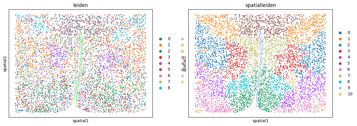
We can see how Leiden clustering identifies cell types while SpatialLeiden defines domains of the tissue.

Resolution search

If you already know how many domains you expect in your sample you can use the spatialleiden.search_resolution() function to identify the resolutions needed to obtain the correct number of clusters.

Conceptually, this function first runs Leiden clustering multiple times while changing the resolution to identify the value leading to the desired number of clusters. Next, this procedure is repeated by running SpatialLeiden, but now the resolution of the latent layer (gene expression) is kept fixed and the resolution of the spatial layer is varied.

n_clusters = adata.obs["domain"].nunique()

latent_resolution, spatial_resolution = sl.search_resolution(
    adata,
    n_clusters,
    latent_kwargs={"seed": seed},
    spatial_kwargs={"layer_ratio": 1.8, "seed": seed, "directed": (False, True)},
)

print(f"Latent resolution: {latent_resolution:.3f}")
print(f"Spatial resolution: {spatial_resolution:.3f}")

Latent resolution: 0.300
Spatial resolution: 1.325

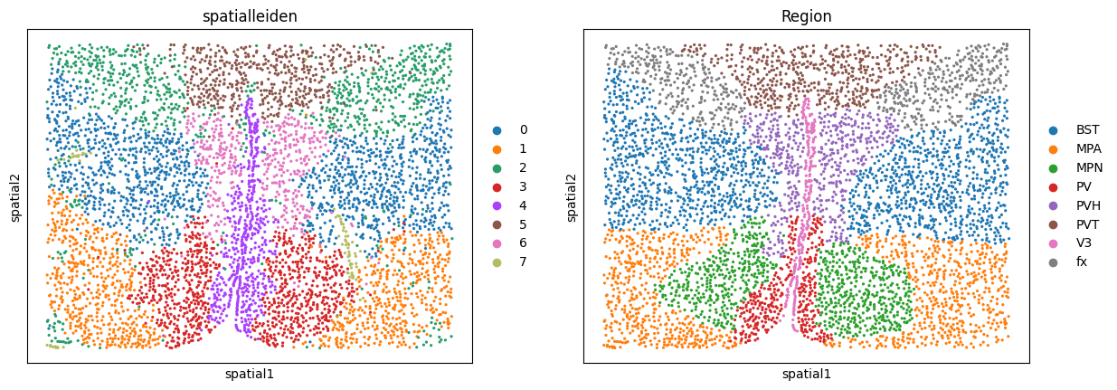
In our case we can compare the resulting clusters to the annotated ground truth regions. If we are not satisfied with the results, we can go back and tweak other parameters such as the underlying neighborhood graphs or the layer_ratio to achieve the desired granularity of our results.

sc.pl.embedding(adata, basis="spatial", color=["spatialleiden", "Region"])