Usage

To demonstrate the usage of the spatialleiden package we are going to use a MERFISH data set from Moffit et al. 2018 that can be downloaded from figshare and then loaded as anndata.AnnData object.

Show code cell content

Hide code cell content

from tempfile import NamedTemporaryFile
from urllib.request import urlretrieve

import anndata as ad

with NamedTemporaryFile(suffix=".h5ad") as h5ad_file:
    urlretrieve("https://figshare.com/ndownloader/files/40038538", h5ad_file.name)
    adata = ad.read_h5ad(h5ad_file)


# This is not recommended! Suppressing the warnings is only done because the code is run
# when building the docs and would clutter the webpage
import warnings

warnings.filterwarnings("ignore")

First of all we are going to load the relevant packages that we will be working with as well as setting a random seed that we will use throughout this example to make the results reproducible.

import scanpy as sc
import spatialleiden as sl
import squidpy as sq

random_state = 42

The data set consists of 155 genes and ~5,500 cells including their annotation for the cell type as well as domains.

SpatialLeiden

We will do some standard preprocessing by log-transforming the data and then using PCA for dimensionality reduction. The PCA will be used to build a kNN graph in the latent gene expression space. This graph is the basis for the Leiden clustering.

sc.pp.log1p(adata)
sc.pp.pca(adata, random_state=random_state)

sc.pp.neighbors(adata, random_state=random_state)

Building spatial neighbor graphs

For SpatialLeiden we need an additional graph representing the neighbors in space i.e. which cells are close/next to each other.

What kind of spatial neighbor graph is suitable for the analysis is dependent on the technology used to generate the data. Most of the neighborhood structures interesting for our use cases can be calculated using squidpy.gr.spatial_neighbors().

Generally, if the data is generated from a method with a regular lattice it is advisible to use this for the analysis;

• isometric grid (hexagonal): for Visium with squidpy.gr.spatial_neighbors(adata, coord_type="grid", n_neighs=6)

• square grid: for binned Stereo-seq and VisiumHD with squidpy.gr.spatial_neighbors(adata, coord_type="grid", n_neighs=4) (using 8 neighbors is also possible)

If your data does not originate from a regular lattice, there are various options to build your neighborhood graph. This applies to all imaging-based methodologies that are usually analysed after segmenting cells, but also technolgoies with regular lattices if you use cell segmentation (such as Stereo-seq or VisiumHD).

• kNN: calculating the k-nearest neighbors per cell with squidpy.gr.spatial_neighbors(adata, coord_type="generic", n_neighs=k)

• Delaunay triangulation: squidpy.gr.spatial_neighbors(adata, coord_type="generic", delaunay=True)

• radius-based: with a threshold of r units squidpy.gr.spatial_neighbors(adata, coord_type="generic", radius=r)

• other methods such as Gabriel graphs, …

For the neighborhoods that are not based on regular grids we can, furthermore, scale the weight of each edge bsaed on the distance between the two cells (that’s why it is not useful for the regular grid case as the neighbors will be equidistant). This can be achieved by calculating connectivities based on the distances using the spatialleiden.distance2connectivity() function.

Here, we will use a kNN graph with 10 neighbors.

sq.gr.spatial_neighbors(adata, coord_type="generic", n_neighs=10)

adata.obsp["spatial_connectivities"] = sl.distance2connectivity(
    adata.obsp["spatial_distances"]
)

Finding clusters

Now, we can already run spatialleiden.spatialleiden() (which we will also compare to normal Leiden clustering).

The layer_ratio determines the weighting between the gene expression and the spatial layer and is influenced by the graph structures (i.e. how many connections exist, the edge weights, etc.); the lower the value is the closer SpatialLeiden will be to normal Leiden clustering, while higher values lead to more spatially homogeneous clusters.

The resolution has the same effect as in Leiden clustering (higher resolution will lead to more clusters) and can be defined for each of the layers (but for now is left at its default value).

sc.tl.leiden(adata, directed=False, random_state=random_state)

sl.spatialleiden(
    adata, layer_ratio=1.8, directed=(False, True), random_state=random_state
)

sc.pl.embedding(adata, basis="spatial", color=["leiden", "spatialleiden"])

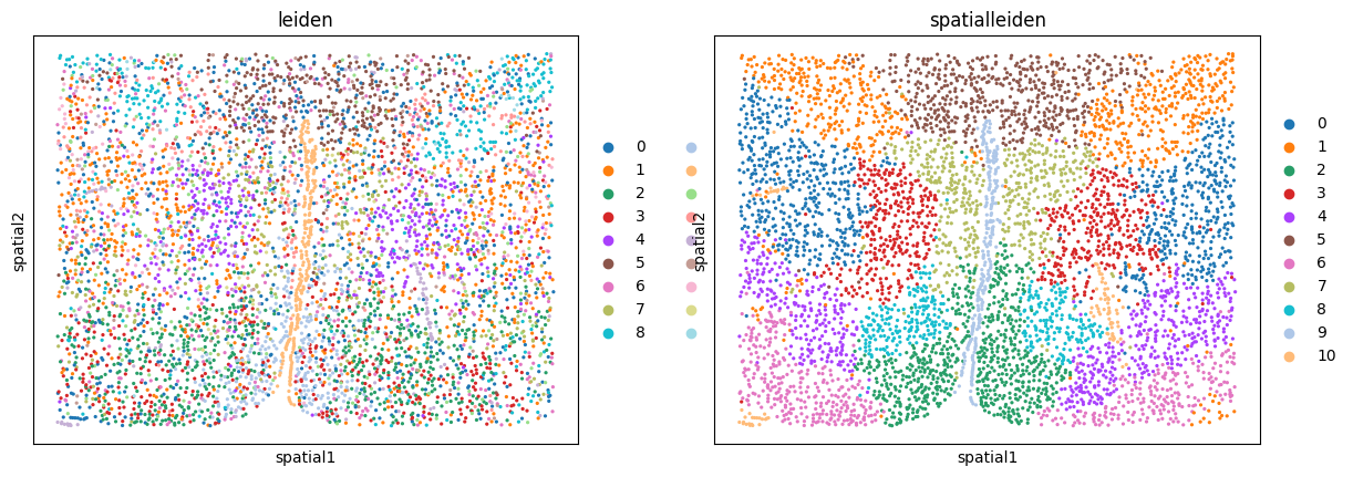
We can see how Leiden clustering identifies cell types while SpatialLeiden defines domains of the tissue.

Resolution search

If you already know how many domains you expect in your sample you can use the spatialleiden.search_resolution() function to identify the resolutions needed to obtain the correct number of clusters.

Conceptually, this function first runs Leiden clustering multiple times while changing the resolution to identify the value leading to the desired number of clusters. Next, this procedure is repeated by running SpatialLeiden, but now the resolution of the latent layer (gene expression) is kept fixed and the resolution of the spatial layer is varied.

n_clusters = adata.obs["domain"].nunique()

latent_resolution, spatial_resolution = sl.search_resolution(
    adata,
    n_clusters,
    latent_kwargs={"random_state": random_state},
    spatial_kwargs={
        "layer_ratio": 1.8,
        "random_state": random_state,
        "directed": (False, True),
    },
)

print(f"Latent resolution: {latent_resolution:.3f}")
print(f"Spatial resolution: {spatial_resolution:.3f}")

Latent resolution: 0.300
Spatial resolution: 1.325

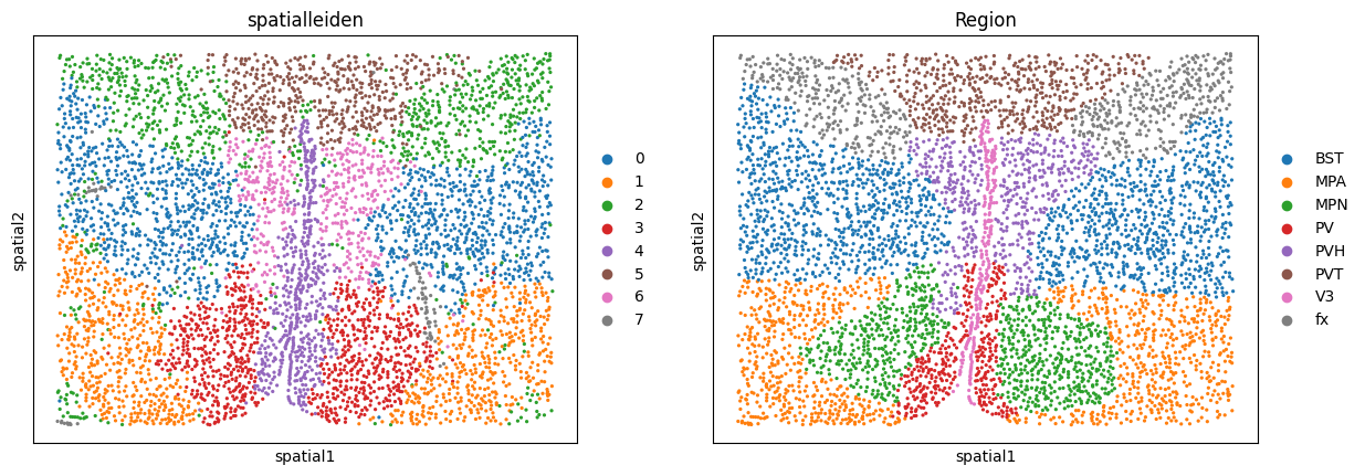
In our case we can compare the resulting clusters to the annotated ground truth regions. If we are not satisfied with the results, we can go back and tweak other parameters such as the underlying neighborhood graphs or the layer_ratio to achieve the desired granularity of our results.

Show code cell content

Hide code cell content

# needed for scanpy v1.11 otherwise plotting fails because the number of clusters changed
del adata.uns["spatialleiden_colors"]

sc.pl.embedding(adata, basis="spatial", color=["spatialleiden", "Region"])